2 Usage¶

2.1 Basic usage¶

The most common use case for symlens is to get noise curves for lensing, and to run lensing reconstruction on CMB maps. We will cover this first, and later come to custom estimators that exploit the full power and flexibility of this package.

2.1.1 Geometry¶

Skip this if you are familiar with the pixell library. Most functions that return something immediately useful take a shape,``wcs`` pair as input. In short, this pair specifies the footprint or geometry of the patch of sky on which calculations are done. If you are playing with simulations or just want quick forecasts, you can make your own shape,``wcs`` pair as follows:

>>> from pixell import enmap
>>> shape,wcs =
enmap.geometry(shape=(2048,2048),res=np.deg2rad(2.0/60.),pos=(0,0))

to specify a footprint consisting of 2048 x 2048 pixels of width 2 arcminutes and centered on the origin of a CEA geometry.

All outputs are 2D arrays in Fourier space, so you will need some way to bin it in annuli. A map of the absolute wavenumbers is useful for this

>>> modlmap = enmap.modlmap(shape,wcs)

To read a map in from disk and get its geometry, you could do

>>> imap = enmap.read_map(fits_file_name)
>>> shape,wcs = imap.shape, imap.wcs

Please read the documentation for pixell for more information.

2.1.2 Noise curves¶

Using the machinery described in Custom estimators below, a number of pre-defined mode-coupling noise curves have been built. We provide some examples of using these. All of these require a shape,``wcs`` geometry pair as described above. Next, you also need to have a Fourier space mask at hand that enforces what multipoles in the CMB map are included.

A convenience function is provided for generating simple Fourier space masks. e.g.

>>> from symlens import utils
>>> tellmin = 100
>>> tellmax = 3000
>>> kmask = utils.mask_kspace(shape,wcs,lmin=tellmin,lmax=tellmax)

Finally, you also need a feed_dict, a dictionary which maps names of variables (keys) to 2D arrays containing data, filters, etc. which are fed in at the very final integration step. With custom estimators described later, you get to choose the names of your variables. But the convenience of the canned functions described here comes with the cost of having to learn what variable convention is defined inside them. We will learn by example.

Lensing noise curves require CMB power spectra. The naming convention for the feed_dict for these is:

uC_X_Y for CMB XY spectra that go in the lensing response function, e.g. uC_T_T for the TT spectrum (despite the notation, this should be the lensed spectrum, not the unlensed spectrum)
tC_X_Y for total CMB XY spectra that go in the lensing filters. e.g. tC_T_T for the total TT spectrum that includes beam-deconvolved noise.

These have to be specified on the 2D Fourier space grid. We can build them like this:

>>> feed_dict = {}
>>> feed_dict['uC_T_T'] = utils.interp(ells,ctt)(modlmap)
>>> feed_dict['tC_T_T'] = utils.interp(ells,ctt)(modlmap)+(33.*np.pi/180./60.)**2./utils.gauss_beam(modlmap,7.0)**2.

where I’ve used the convenience function interp to interpolate an ells,``cltt`` 1D spectrum specification isotropically on to the Fourier space grid, and created a Planck-like total beam-deconvolved spectrum using the gauss_beam function. That’s it! Now we can get the pre-built Hu Okamoto 2001 (estimator=”hu_ok”) noise for the TT lensing estimator as follows,

>>> import symlens as s
>>> nl2d = s.N_l(shape,wcs,feed_dict,"hu_ok","TT",xmask=kmask,ymask=kmask)

which can be binned in annuli to obtain a lensing noise curve.

2.1.3 Lensing maps¶

To make a lensing map, we need to provide beam deconvolved Fourier maps of the CMB, which for a quadratic estimator <XY> have default variable names of X and Y,

>>> feed_dict['X'] = beam_deconvolved_fourier_T_map
>>> feed_dict['Y'] = beam_deconvolved_fourier_T_map

An important thing to remember is that by default, the code expects “physical” normalization of FFTs in pixell (not the default normalization in pixell), i.e. you should be passing in Fourier maps that come from something like

>>> beam_deconvolved_fourier_T_map = enmap.fft(imap,normalize='phys')

or

>>> beam_deconvolved_fourier_T_map = enmap.map2harm(imaps,normalize='phys')[0]

One can then obtain the unnormalized lensing map simply by doing,

>>> ukappa = s.unnormalized_quadratic_estimator(shape,wcs,
                        feed_dict,"hu_ok","TT",xmask=kmask,ymask=kmask)

and also obtain its normalization,

>>> norm = s.A_l(shape,wcs,feed_dict,"hu_ok","TT",xmask=kmask,ymask=kmask)

and combine into a normalized Fourier space CMB lensing convergence map,

>>> fkappa = norm * ukappa

2.1.4 General noise curves¶

To perform more complicated calculations like cross-covariances, noise for non-optimal estimators, mixed experiment estimators (for gradient cleaning), split-based lensing N0 curves, etc., we need to learn how to attach field names, which make the feed_dict expect more variables than what was described earlier.

Let’s first show how we can obtain a general noise cross-covariance. We can for example obtain the same TT lensing noise curve as above but in a more round-about way by asking what the cross-covariance of the TT estimator is with the TT estimator itself,

>>> Nl =
N_l_cross(shape,wcs,feed_dict,alpha_estimator="hu_ok",alpha_XY="TT",
                             beta_estimator="hu_ok",beta_XY="TT",
                             xmask=kmask,ymask=kmask)

This works just like before. However, what if the instrument noise in the first leg of the estimator is uncorrelated with the noise in the second leg? Then, we need to differentiate between the four fields that appear above. We can do that by providing names for these fields.

>>> Nl = N_l_cross(shape,wcs,feed_dict,
             alpha_estimator="hu_ok",alpha_XY="TT",
             beta_estimator="hu_ok",beta_XY="TT",
             xmask=kmask,ymask=kmask,
             field_names_alpha=['E1','E2'],
             field_names_beta=['E1','E2'])

This modifies the total power spectra variable names that feed_dict expects. The above command will not work unless tC_E1_T_E1_T, tC_E2_T_E2_T, tC_E1_T_E2_T, tC_E2_T_E1_T are also provided, instead of just the usual tC_T_T. Specifying these in feed_dict allows one to generalize to a wider variety of estimators.

2.1.5 Other built-in estimators¶

The following are currently available:

Hu Okamoto 2001 TT, TE, EE, EB, TB
Hu DeDeo Vale 2007 TT, TE, ET, EE, EB, TB
Schaan, Ferraro 2018 shear TT

For the shear estimator, the built-in variable scheme also expects duC_T_T , the logarithmic derivative of the lensed CMB temperature,

>>> feed_dict['duC_T_T'] =
    utils.interp(ells,np.gradient(np.log(lcltt),np.log(ells)))(modlmap)

Once this is added to feed_dict, noise curves and shear maps can be obtained as before,

>>> Nl = s.N_l(shape,wcs,feed_dict,"shear","TT",
          xmask=tmask,ymask=tmask)
>>> Al = s.A_l(shape,wcs,feed_dict,"shear","TT",xmask=tmask,ymask=tmask)
>>> ushear = s.unnormalized_quadratic_estimator(shape,wcs,feed_dict,"shear","TT",xmask=tmask,ymask=tmask)
>>> shear = Al * ushear

2.2 Custom estimators¶

We can build general factorizable quadratic estimators as follows.

We need to specify the mode coupling form (little f):

$f(\vec{l}_1,\vec{l}_2)$

and specify the filter form (big F):

$F(\vec{l}_1,\vec{l}_2)$

For reference, these are related to the quadratic estimator,

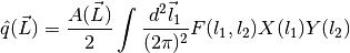
$\hat{q}(\vec{L}) = \frac{A(\vec{L})}{2} \int \frac{d^2\vec{l}_1}{(2\pi)^2} F(l_1,l_2) X(l_1) Y(l_2)$

and normalization,

$A(\vec{L}) = L^2 \left[\int \frac{d^2\vec{l}_1}{(2\pi)^2} F(l_1,l_2) f(l_1,l_2)\right]^{-1}$

where $\vec{L}=\vec{l}_1 + \vec{l}_2$ .

The expressions $f(\vec{l}_1,\vec{l}_2)$ and $F(\vec{l}_1,\vec{l}_2)$ must be specified in terms of the following special symbols:

Ldl1 for $\vec{L}.\vec{l_1}$
Ldl2 for $\vec{L}.\vec{l_2}$
cos2t12 for $\mathrm{cos}(2\theta_{12})$
sin2t12 for $\mathrm{sin}(2\theta_{12})$
L for $|\vec{L}|$

and any other arbitrary symbols which will be replaced with numerical data later on.

The special symbols can be accessed directly from the module, e.g.:

>>> import symlens as s
>>> s.Ldl1
>>> s.L
>>> s.cost2t12

and arbitrary symbols can be defined either as functions of l1 or of l2, using a wrapper in the module:

>>> s.e('X_l1')
>>> s.e('Y_l2')

The ‘_l1’ or ‘_l2’ suffix for arbitrary symbols is critical for the factorizer to know. With these, a large variety of estimators and noise functions can be built, including lensing, magnification, shear, birefringence, patchy tau, mixed estimators (for gradient cleaning), split lensing estimators, etc.

e.g., we can build an integrand for the Hu, Okamoto 2001 TT lensing estimator normalization as follows,

# Build HuOk TT estimator integrand
>>> f = s.Ldl1 * s.e('uC_T_T_l1') + s.Ldl2 * s.e('uC_T_T_l2')
>>> F = f / 2 / s.e('tC_T_T_l1') / s.e('tC_T_T_l2')
>>> expr1 = f * F # this is the integrand

We then provide data arrays for use after factorization in feed_dict. These are lensed TT spectra interpolated on to 2D Fourier space.

>>> feed_dict = {}
>>> feed_dict['uC_T_T'] = utils.interp(ells,ctt)(modlmap)
>>> feed_dict['tC_T_T'] = utils.interp(ells,ctt)(modlmap)

For the integral to be sensible, we must also mask regions in Fourier space we don’t want to include.

>>> tellmin = 10 ; tellmax = 3000
>>> xmask = utils.mask_kspace(shape,wcs,lmin=tellmin,lmax=tellmax)

With these in hand, we can call the core function in symlens for the factorized integral.

>>> integral = s.integrate(shape,wcs,feed_dict,expr1,xmask=xmask,ymask=xmask).real